Production + Research Project

4D Auto-Labeling & Pure LiDAR 3D Detection

Two eras of autonomous-driving auto-labeling — a Tesla-inspired vision-only 4D pipeline, then a multi-modal and pure-LiDAR 3D detection system.

Timeline: 2022.11–2024
Context: Hozon Auto × SJTU IRMV · PhiGent Robotics
Role: Perception Team Leader · 3D Perception Algorithm Engineer
Stage: Production & R&D

Overview

What is this project about?

A two-phase journey in autonomous-driving auto-labeling: first a Tesla-AI-Day-inspired vision-only 4D auto-labeling pipeline with Hozon Auto and SJTU IRMV, then a multi-modal 4D auto-labeling and production pure-LiDAR 3D detection system at PhiGent Robotics — optimized at the data, model, and loss levels.

production research 3d-4d perception deployment

Same Direction, Two Eras

From vision-only 4D labels to pure-LiDAR detection

Both phases share one goal — automatically producing high-quality 4D training labels for autonomous driving — but differ in era, team, and sensor stack. The timeline below moves from a Tesla-inspired vision-only pipeline to a multi-modal + pure-LiDAR production system.

Logic map

One goal, two eras — vision-only 4D, then multi-modal + pure LiDAR

Both lanes chase the same prize: high-quality 4D labels with no human in the loop. Hover a node to compare the eras.

01 2022.11 – 2023.04 Hozon Auto × SJTU IRMV Perception Team Leader

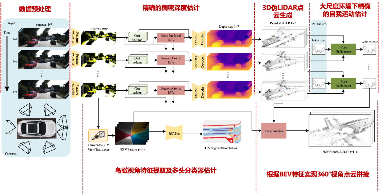
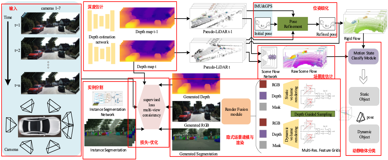
Video Offline 4D Auto-Labeling

A vision-only offline pipeline replicating the spirit of Tesla AI Day: from multi-camera video + IMU, estimate surround depth, lift to a 360° pseudo-LiDAR, separate static and dynamic, and fuse everything into a 4D scene.

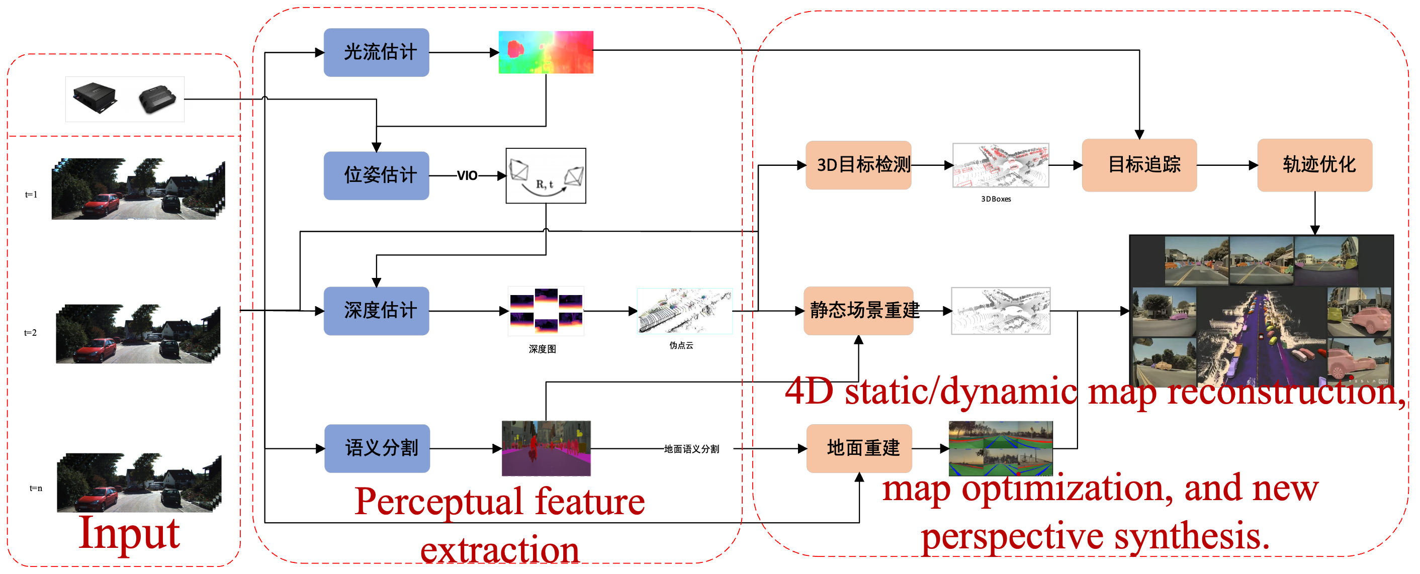
System pipeline. Multi-camera + IMU → parallel perception features (flow / pose / depth / semantics) → three branches (3D detection · static reconstruction · ground reconstruction) → a fused 4D scene with novel-view synthesis.

Step 1 · Depth

Surround-view depth → pseudo-LiDAR

Multi-frame cost volume + Conv-LSTM + BEV fusion → 360° pseudo-LiDAR; IMU/GPS pose refinement

Step 2 · Features

Perceptual features → motion state

Optical flow · semantic/instance seg · scene flow → classify each point dynamic / static

Step 3A · Static

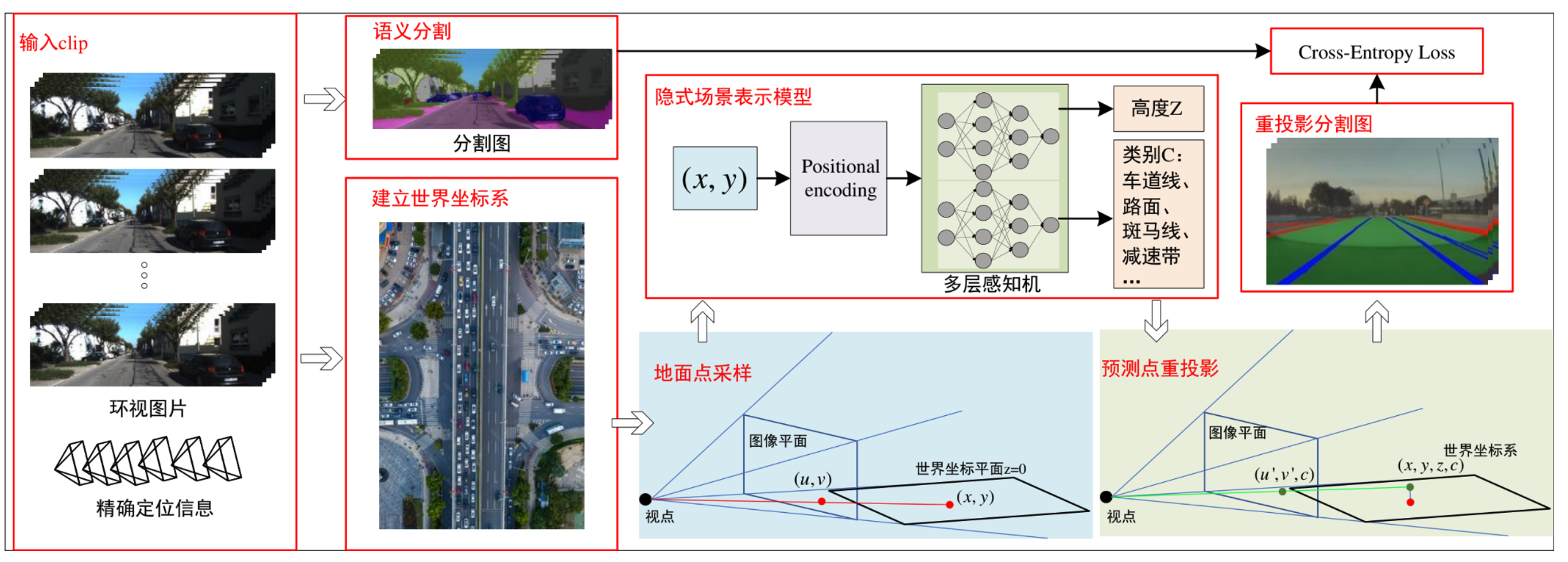
Scene reconstruction

Warp multi-frame → global map; NeRF implicit ground + novel views

Step 3B · Dynamic

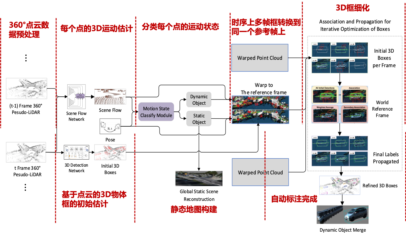
3D box labeling

Per-point scene flow → align frames → associate & weighted-average 3D boxes

Step 4 · Fuse

4D auto-labels

HD-map + 3D tracks + segmentation + synthetic views → time × space × semantics × motion

Foundation: pseudo-LiDAR

Surround-view depth estimation network — Surround-view depth → 360° pseudo-LiDAR, the geometric base for 4D reconstruction.

Static element reconstruction pipeline — **Static elements.** Instance segmentation + implicit (NeRF-style) rendering, separated by depth-guided scene flow.

Dynamic 3D box labeling pipeline — **Dynamic objects.** Scene-flow motion classification → cross-frame association → refined 3D boxes.

NeRF-based simulation data synthesis — **Simulation synthesis.** Implicit MLP predicts height & semantics; reprojection + cross-entropy drives high-quality synthetic labels.

Deep-dive walkthrough. The design, logic, and a breakdown of a Tesla-style visual 4D auto-labeling system.

02 2024 · Internal R&D PhiGent Robotics 3D Perception Algorithm Engineer

4D Auto-Labeling & Pure LiDAR 3D Detection

Moving to a multi-modal stack: harden a BEVFusion-based 4D auto-labeler on hard objects (VRUs, long trailers, far range), then ship a production pure-LiDAR 3D detector on solid-state LiDAR.

Workstream A · Data level

Adaptive VRU instance augmentation

VRUs (pedestrians, cyclists) are safety-critical but heavily under-represented. We build a VRU instance database and adaptively paste real instances into scenes to rebalance training.

VRU instance DB Adaptive paste Image + point-cloud joint align Depth-legal placement

① Collect

Instance mining

Extract every VRU: RGB patch + LiDAR segment + spatial meta (position / depth / pose)

② Database

Layered index

Index by class / distance band / scene type → diverse coverage

③ Fuse

Adaptive paste

Scene depth → legal position; match scale / occlusion; paste into image + point cloud jointly

④ Sync

Label synchronization

Auto-generate 2D BBox / 3D BBox / mask → complete supervision

Copy-paste augmentation

Real-instance copy-paste in image and point cloud — Real VRU instances pasted with geometric consistency across both modalities.

Result. Measurable precision & recall gains on VRU classes after adaptive instance augmentation.

Builds on. Real-instance paste from Real-Aug and adaptive geometric alignment from PGT-Aug (NeurIPS 2024), extended to joint Camera + LiDAR placement with depth-legal constraints and dynamic sampling.

Workstream B · Model level

BEV range & resolution tuning

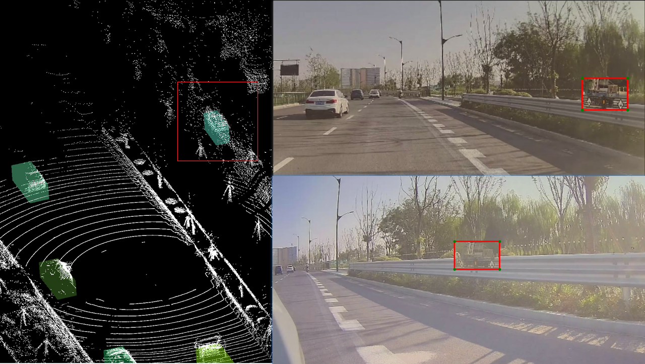
Clamp the perception range to ≤ 210 m and raise BEV resolution, so far-field features stay dense — directly improving very-long-range 3D detection during training and release.

Before

Range > 210 m

Low BEV resolution

Far-field features sparse → weak long-range recall

After

Range ≤ 210 m

High BEV resolution

Far-field features dense → stronger long-range 3D detection

Workstream C · Loss level

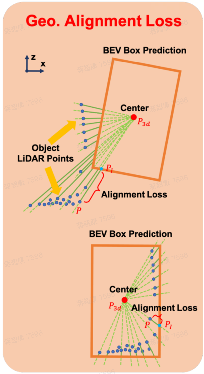
Ultra-long trailer: geometry-alignment loss

Articulated trailers bend when turning, so a single box never fits and heading drifts. We add multi-box labeling for multi-section trailers and a loss that forces box boundaries to hug the LiDAR surface.

Multi-box labeling Point-to-boundary loss Heading correction

Problem

Articulated & occluded

Tractor + trailer 1 + trailer 2 … each section a different angle → single box distorts IoU; sparse points

Labeling

Multi-box supervision

Hand-label multi-section trailers so the model learns to emit several boxes per vehicle

Loss

Point-to-boundary alignment

For each LiDAR point P: cast a ray from box center through P
Ray ∩ box boundary = P_l → Loss = dist(P, P_l)
Point outside → loss rotates/translates the box onto the cloud; aligned → loss → 0

Result

Tight, correctly-oriented boxes

Boxes hug the trailer surface; heading error sharply reduced

Geometry-alignment loss

Point-to-boundary geometry loss construction — Top: heading too large → loss pulls the box. Bottom: aligned → loss ≈ 0.

Trailer heading prediction failures — **Before.** Boxes miss the trailer body with large heading errors.

Automatic 3D detection and labeling result — **After.** Stable, tightly-fitted automatic 3D detection and labeling.

Workstream D · Production · Seyond Falcon K1

Pure LiDAR 3D detection

A production 3D detector for solid-state LiDAR — an open pipeline redesigned around reflectivity features and dilated convolutions, tuned for the sparse far field.

Reflectivity feature Dilation FPN CenterHead · NMS-free INT8 · Orin

01 · Preprocess

Point-cloud preparation

Range filter → RANSAC ground removal → reflectivity normalize → pillar voxelization

02 · Pillars

PillarFeatureNet

Feature [x,y,z,intensity,x_c,y_c,z_c,x_p,y_p]; reflectivity is the core cue; hash voxelization + INT8 MLP

03 · Scatter

Sparse → dense BEV

CUDA scatter via pillar-coordinate hash → dense pseudo-image (~35% faster end-to-end)

04 · Backbone

SECOND + Dilation FPN

Dilated deconv d = 1,2,4 enlarges receptive field for sparse far-field context

05 · Head

CenterHead

Center heatmap (GaussianFocalLoss) + regression (offset / z / size / rotation / velocity); NMS-free peak extraction

Algorithm framework

Pure LiDAR 3D detection framework — Solid-state-LiDAR detector: pillars → scatter → SECOND + Dilation FPN → CenterHead.

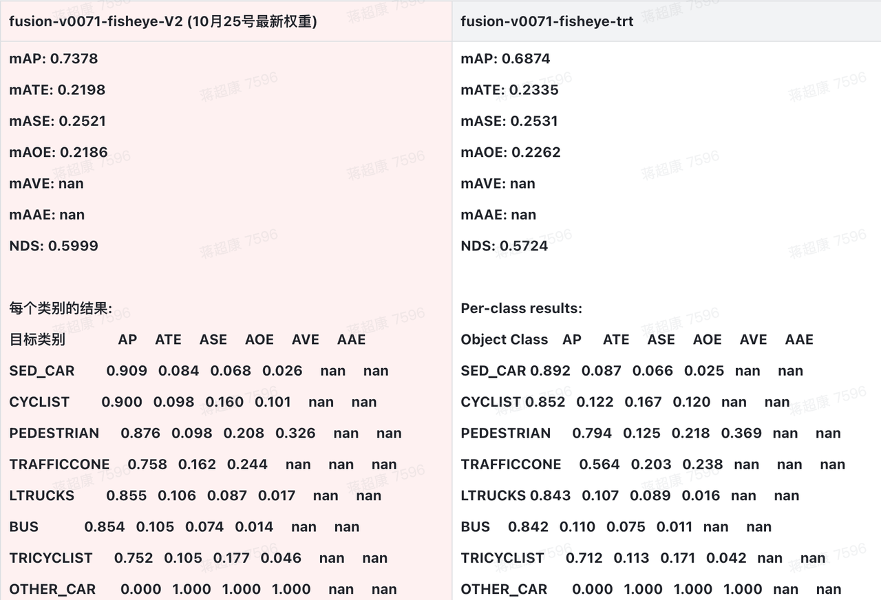
Ablation · mAP by class

What each idea contributes

Method	mAP	Car	Bicycle	Pedestrian	Cone	Truck	Bus	Tricycle
Pillar features (baseline)	0.667	0.959	0.835	0.710	0.722	0.628	0.863	0.615
+ Reflectivity	0.704	0.966	0.861	0.780	0.787	0.653	0.873	0.715
+ Dilation FPN	0.719	0.964	0.865	0.793	0.819	0.701	0.887	0.722
Voxel sparse features	0.714	0.954	0.874	0.838	0.844	0.586	0.839	0.775
Reflectivity + dilated conv (final)	0.763	0.968	0.909	0.885	0.907	0.780	0.892	0.760

Confidentiality note. Only public-level pipeline structure is shown. Internal datasets, labeling rules, exact metrics, model parameters, and customer-specific details are omitted; thresholds are illustrative.